Linear Regression, Multiple and Polynomial Regression - A Statistical Approach

In statistics, linear regression is a linear approach to modelling the relationship between a scalar response and one or more explanatory variables (also known as dependent and independent variables). The case of one explanatory variable is called simple linear regression; for more than one, the process is called multiple linear regression. This term is distinct from multivariate linear regression, where multiple correlated dependent variables are predicted, rather than a single scalar variable.

In linear regression, the relationships are modelled using linear predictor functions whose unknown model parameters are estimated from the data. Such models are called linear models. Most commonly, the conditional mean of the response given the values of the explanatory variables (or predictors) is assumed to be an affine function of those values; less commonly, the conditional median or some other quantile is used. Like all forms of regression analysis, linear regression focuses on the conditional probability distribution of the response given the values of the predictors, rather than on the joint probability distribution of all of these variables, which is the domain of multivariate analysis.

Why Linear Regression?

Linear Regression helps us to understand more about the data and help us predict what the next data might be. Now, it has many disadvantages but it may correctly predict data that is very simple yet complex to human eyes.

Packages Required to run codes in Python

Use pip install matplotlib and pip install numpy in the terminal to install these libraries. Make sure you have Python installed.

Simple Linear Regression

Before we proceed to the code, let's do some mathematical theory first.

• It's also known as the line of best fit.

• Supervised X→Y.

• Regression output is a number

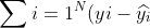
The line of best fit is given by

Error is

 align="left")

Correct Error Prediction

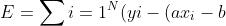)^{2} align="left")

Therefore to minimize errors,

&

would be 0.

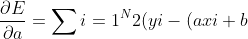)(-x{i}) align="left")

&

or,

or,

...(1)

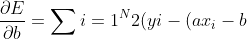)(-1)=0 align="left")

&

or,

or,

...(2)

Now after solving Eqn 1 & 2,

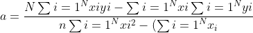^{2}} align="left")

and

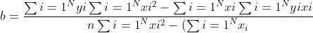^{2}} align="left")

After Substituting sample means,

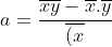^{2}}-(\overline{x})^{2}} align="left")

and

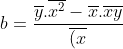^{2}}-(\overline{x})^{2}} align="left")

Note:(In case you are wondering what sample mean means)

The R-Squared Value is the value by which we determine how good the model is.
We can compute this by,

Where

^{2} align="left")

and

^{2} align="left")

Things to Note:

• If the R-squared value is close to 1, the model is good

• If the R-squared value is close to 0, the model is average

• If the R-squared value is less than 0 or greater than 1, the model is very bad

Now, the Python Code (Download the dataset here:data_1d.csv)
# shows how linear regression analysis can be applied to 1-dimensional data import numpy as np import matplotlib.pyplot as plt # load the data X = [] Y = [] for line in open('data_1d.csv'): x, y = line.split(',') X.append(float(x)) Y.append(float(y)) # let's turn X and Y into numpy arrays since that will be useful later X = np.array(X) Y = np.array(Y) # let's plot the data to see what it looks like plt.scatter(X, Y)plt.show() # apply the equations we learned to calculate a and b # denominator is common # note: this could be more efficient if # we only computed the sums and means once denominator = X.dot(X) - X.mean() * X.sum() a = ( X.dot(Y) - Y.mean()*X.sum() ) / denominator b = ( Y.mean() * X.dot(X) - X.mean() * X.dot(Y) ) / denominator # let's calculate the predicted Y Yhat = a*X + b # let's plot everything together to make sure it worked plt.scatter(X, Y) plt.plot(X, Yhat)plt.show() # determine how good the model is by computing the r-squared d1 = Y - Yhat d2 = Y - Y.mean() r2 = 1 - d1.dot(d1) / d2.dot(d2) print("the r-squared is:", r2)

Here is a picture of data represented in a plot:-

And now, we draw a linear regression line:-

Here is the r-squared value for our model:-

r-squared is: 0.9911838202977805

Moore's Law

It's also called the first line of attack to discover correlations in data. Take an example:- Transistor count on IC doubles every 2 years , , ... (Exponential)
But, (Linear)

Moore Law's Derivation

which can be represented in the form of

...(1)

...(2)
Now divide 2 by 1,

and log r is constant.
Now, the Python Code (Download the dataset here:moore.csv)
# shows how linear regression analysis can be applied to moore's law import re import numpy as np import matplotlib.pyplot as plt X = [] Y = [] # some numbers show up as 1,170,000,000 (commas) # some numbers have references in square brackets after them non_decimal = re.compile(r'[^\d]+') for line in open('moore.csv'): r = line.split('\t') x = int(non_decimal.sub('', r[2].split('[')[0])) y = int(non_decimal.sub('', r[1].split('[')[0])) X.append(x) Y.append(y) X = np.array(X) Y = np.array(Y) plt.scatter(X, Y)plt.show() Y = np.log(Y) plt.scatter(X, Y)plt.show() # copied from lr_1d.py denominator = X.dot(X) - X.mean() * X.sum() a = ( X.dot(Y) - Y.mean()*X.sum() ) / denominator b = ( Y.mean() * X.dot(X) - X.mean() * X.dot(Y) ) / denominator # let's calculate the predicted Y Yhat = a*X + b plt.scatter(X, Y) plt.plot(X, Yhat)plt.show() # determine how good the model is by computing the r-squared d1 = Y - Yhat d2 = Y - Y.mean() r2 = 1 - d1.dot(d1) / d2.dot(d2) print("a:", a, "b:", b) print("the r-squared is:", r2) # how long does it take to double? # log(transistorcount) = a*year + b # transistorcount = exp(b) * exp(a*year) # 2*transistorcount = 2 * exp(b) * exp(a*year) = exp(ln(2)) * exp(b) * exp(a * year) = exp(b) * exp(a * year + ln(2))
# a*year2 = a*year1 + ln2 # year2 = year1 + ln2/a print("time to double:", np.log(2)/a, "years")

Here is a visualization of the data:-

Now we convert to logarithmic scale:-

Draw a linear regression line in the scaled data:-

And the output of the code-

a: 0.35104357336499337 b: -685.0002843816548 the r-squared is: 0.9529442852285758 time to double: 1.974533172379868 years

Multiple Linear Regression

Multiple linear regression (MLR), also known simply as multiple regression, is a statistical technique that uses several explanatory variables to predict the outcome of a response variable. The goal of multiple linear regression (MLR) is to model the linear relationship between the explanatory (independent) variables and the response (dependent) variable.

In essence, multiple regression is the extension of ordinary least-squares (OLS) regression that involves more than one explanatory variable.

Formula and Calculation of Multiple Linear Regression:

where for i=n observations,
\= dependent variable
\= explanatory variables
\= y-intercept(constant term)
\= slope coeffs for each explanatory variable
\= the model's error term

The multiple regression model is based on the following assumptions:

• There is a linear relationship between the dependent variables and the independent variables.

• The independent variables are not too highly correlated with each other.

• yi observations are selected independently and randomly from the population.

• Residuals should be normally distributed with a mean of 0 and variance σ.

The R-squared value is the same for Multiple Linear Regression and Linear Regression.
Now, the Python Code (Download the dataset here:data_2d.csv)
# shows how linear regression analysis can be applied to 2-dimensional data import numpy as np from mpl_toolkits.mplot3d import Axes3D import matplotlib.pyplot as plt # load the data X = [] Y = [] for line in open('data_2d.csv'): x1, x2, y = line.split(',') X.append([float(x1), float(x2), 1]) # add the bias term Y.append(float(y)) # let's turn X and Y into numpy arrays since that will be useful later X = np.array(X) Y = np.array(Y) # let's plot the data to see what it looks like fig = plt.figure() ax = fig.add_subplot(111, projection='3d') ax.scatter(X[:,0], X[:,1], Y)plt.show() # apply the equations we learned to calculate a and b # numpy has a special method for solving Ax = b # so we don't use x = inv(A)*b # note: the * operator does element-by-element multiplication in numpy # np.dot() does what we expect for matrix multiplication w = np.linalg.solve(np.dot(X.T, X), np.dot(X.T, Y)) Yhat = np.dot(X, w) # determine how good the model is by computing the r-squared d1 = Y - Yhat d2 = Y - Y.mean() r2 = 1 - d1.dot(d1) / d2.dot(d2) print "the r-squared is:", r2

Here is a 3-D plot of our data:-

And the r-squared value:-

the r-squared is: 0.9980040612475778

Polynomial Regression

Now, the Python Code (Download the dataset here:data_poly.csv)
# shows how linear regression analysis can be applied to polynomial data import numpy as np import matplotlib.pyplot as plt # load the data X = [] Y = [] for line in open('data_poly.csv'): x, y = line.split(',') x = float(x) X.append([1, x, x*x]) # add the bias term x0 = 1 Y.append(float(y)) # let's turn X and Y into numpy arrays since that will be useful later X = np.array(X) Y = np.array(Y) # let's plot the data to see what it looks like plt.scatter(X[:,1], Y)plt.show() # apply the equations we learned to calculate a and b # numpy has a special method for solving Ax = b # so we don't use x = inv(A)*b # note: the * operator does element-by-element multiplication in numpy # np.dot() does what we expect for matrix multiplication w = np.linalg.solve(np.dot(X.T, X), np.dot(X.T, Y)) Yhat = np.dot(X, w) # let's plot everything together to make sure it worked plt.scatter(X[:,1], Y) plt.plot(sorted(X[:,1]), sorted(Yhat)) # note: shortcut since monotonically increasing # x-axis values have to be in order since the points # are joined from one element to the next plt.show() # determine how good the model is by computing the r-squared d1 = Y - Yhat d2 = Y - Y.mean() r2 = 1 - d1.dot(d1) / d2.dot(d2) print("the r-squared is:", r2)

Here is a visualisation of the data:-

And now we draw a polynomial regression line

And the r-squared value:-

the r-squared is: 0.9903457612475679

Exercise

Think you have mastered Regression? Download this dataset and find the best regression for the given dataset.
Download Here:-mlro2.xls
Solution:
# need to sudo pip install xlrd to use pd.read_excel # The data (X1, X2, X3) are for each patient. # X1 = systolic blood pressure # X2 = age in years # X3 = weight in pounds import matplotlib.pyplot as plt import numpy as np import pandas as pd df = pd.read_excel('mlr02.xls') X = df.values # using age to predict systolic blood pressure plt.scatter(X[:, 1], X[:, 0])plt.show() # looks pretty linear! # using weight to predict systolic blood pressure plt.scatter(X[:, 2], X[:, 0])plt.show() # looks pretty linear! df['ones'] = 1 Y = df['X1'] X = df[['X2', 'X3', 'ones']] X2only = df[['X2', 'ones']] X3only = df[['X3', 'ones']] def get_r2(X, Y): w = np.linalg.solve(X.T.dot(X), X.T.dot(Y)) Yhat = X.dot(w) # determine how good the model is by computing the r-squared d1 = Y - Yhat d2 = Y - Y.mean() r2 = 1 - d1.dot(d1) / d2.dot(d2) return r2 print("r2 for x2 only:", get_r2(X2only, Y)) print("r2 for x3 only:", get_r2(X3only, Y)) print("r2 for both:", get_r2(X, Y))

Visit my linear regression GitHub page to get the full programs and all datasets.

Click Here-Codehackerone/linear_regression
Learnt something? Do share this website with your friends.